Building Blocks of Data Systems
Every data system design is assembled from roughly ten building blocks. For each one, know what it’s for, how it works inside, the knobs, and when NOT to use it.
Contents: Message log (Kafka) · Partitioning · Stream processors · Batch engines · Storage & table formats · Serving stores · Caches · Orchestrators · Schema registry · Probabilistic structures
1. The message log (Kafka)
Mental model
A Kafka topic is an append-only, partitioned, replicated log. Producers append; consumers read at their own offset. Data isn’t deleted when it’s read. It’s deleted by retention (time/size) or compaction.
flowchart LR
    P1[Producer A] -->|key=user_1| T0
    P2[Producer B] -->|key=user_2| T1
    P2 -->|key=user_3| T2
    subgraph Topic["Topic: clicks (3 partitions, RF=3)"]
        T0["P0: 0 1 2 3 4 5 →"]
        T1["P1: 0 1 2 3 →"]
        T2["P2: 0 1 2 3 4 →"]
    end
    subgraph CG1["Consumer group: flink-agg"]
        C1[consumer 1]
        C2[consumer 2]
    end
    subgraph CG2["Consumer group: lake-sink"]
        C3[consumer 1]
    end
    T0 --> C1
    T1 --> C2
    T2 --> C2
    T0 --> C3
    T1 --> C3
    T2 --> C3
Key facts interviewers probe
| Concept | What to say |
|---|---|
| Ordering | Guaranteed only within a partition. Same key → same partition (hash(key) % N) → per-key order. |
| Parallelism | Max active consumers in a group = number of partitions. Partitions are the unit of scale. |
| Consumer groups | Each group gets every message once (load-balanced across its members); different groups are independent → fan-out for free. |
| Replication | replication.factor=3, min.insync.replicas=2, producer acks=all → no data loss if one broker dies. |
| Retention | Time/size based (e.g. 7 days) → replay window for reprocessing/backfills. Tiered storage moves old segments to S3 for long retention. |
| Log compaction | Keeps only the latest value per key; tombstone (key, null) deletes. Good for CDC/changelog topics and state restore. |
| Idempotent producer | enable.idempotence=true → broker dedupes retries via (producer id, sequence number). |
| Transactions | Atomic writes across partitions + offset commits → exactly-once for read-process-write within Kafka. |
| Adding partitions | Changes hash(key) % N → breaks key ordering for existing keys. Over-provision up front. |
| Consumer lag | log-end-offset − committed-offset: the health metric for streaming. |
Kafka vs alternatives
| Kafka | Kinesis | Pulsar | Pub/Sub | RabbitMQ/SQS | |
|---|---|---|---|---|---|
| Model | Log | Log (shards) | Log + queue | Managed log-ish | Queue (delete on ack) |
| Replay | ✅ retention | ✅ up to 365d | ✅ tiered | ✅ seek (7d) | ❌ |
| Ordering | per partition | per shard | per key | per ordering key | limited |
| Ops | heavy (or MSK/Confluent) | zero | heavy | zero | light |
| Use when | default for data pipelines | AWS-native, simpler | multi-tenant, geo | GCP-native | task queues, not analytics |
When NOT Kafka: low volume (< a few hundred events/s) where a DB table + CDC or SQS is simpler; pure batch file drops (land in object storage + AutoLoader).
2. Partitioning strategies
Partitioning shows up in Kafka topics, Spark shuffles, table layouts and serving stores. Same trade-off everywhere: locality vs balance.
| Strategy | Example | Pros | Cons |
|---|---|---|---|
| Hash by key | hash(user_id) % 64 | Even spread; co-locates a key’s data (ordering, joins, state) | Hot keys → hot partition; resizing reshuffles |
| Range | dates, A–F, G–M | Range scans, pruning | Hotspots on the “latest” range (time-ordered writes) |
| Round-robin | no key | Perfect balance | No ordering; aggregations need a shuffle later |
| Time-based (tables) | PARTITION BY event_date | Pruning, easy retention/backfill per day | Too fine-grained → small files |
| Composite / salted | (campaign_id, salt 0–9) | Spreads hot keys | Two-phase aggregation needed |
| Geo / tenant | region, tenant_id | Isolation, data residency | Uneven tenant sizes |
Hot-key mitigation (classic deep dive)
flowchart LR
    E[Events<br/>key = campaign_id] --> S{Hot key?}
    S -->|no| H1[hash campaign_id]
    S -->|yes| SALT[append salt 0..N-1<br/>campaign_id#7]
    H1 --> A1[Partial aggregate per key]
    SALT --> A1
    A1 --> M[Second stage:<br/>strip salt, merge partials]
    M --> OUT[(Final per campaign)]
- Detect: per-partition lag/throughput skew; top-K key metrics.
- Salt the hot keys (or all keys) with a random suffix → partial aggregates → merge in a second stage. Works because SUM/COUNT/MIN/MAX/HLL are mergeable.
- Local pre-aggregation (combiner) before shuffle: Spark does this automatically for
reduceByKey/groupBy().agg()partial aggregation. - Split hot keys onto dedicated partitions/consumers.
- In joins: broadcast the small side, or AQE skew join (Spark splits skewed partitions automatically).
3. Stream processors
| Spark Structured Streaming | Apache Flink | Kafka Streams | Managed (DLT, Dataflow) | |
|---|---|---|---|---|
| Model | Micro-batch (default), continuous experimental | True streaming, event-at-a-time | Library inside your app | Spark / Beam under the hood |
| Latency | ~100 ms – seconds (Real-Time Mode lowers this) | ms | ms | seconds |
| State | RocksDB state store, applyInPandasWithState / transformWithState | Best-in-class: keyed state, timers, savepoints | RocksDB, changelog topics | managed |
| Exactly-once | checkpoint + idempotent/transactional sinks | checkpoint barriers (Chandy-Lamport) + 2PC sinks | Kafka transactions | ✅ |
| Batch + stream same code | ✅ (same DataFrame API) | ✅ (Table API) | ❌ | ✅ |
| Choose when | Lakehouse/Delta shop, seconds latency OK, team knows Spark | Sub-second, complex event processing, huge state, timers | Kafka-in Kafka-out microservices | Want zero ops |
Talking point: “Our freshness SLA is under a minute and we’re a Databricks shop, so Structured Streaming with Delta sinks is the pragmatic choice. If we needed sub-100 ms fraud scoring with per-user timers, I’d pick Flink.”
Core streaming concepts (detail in streaming deep dive)
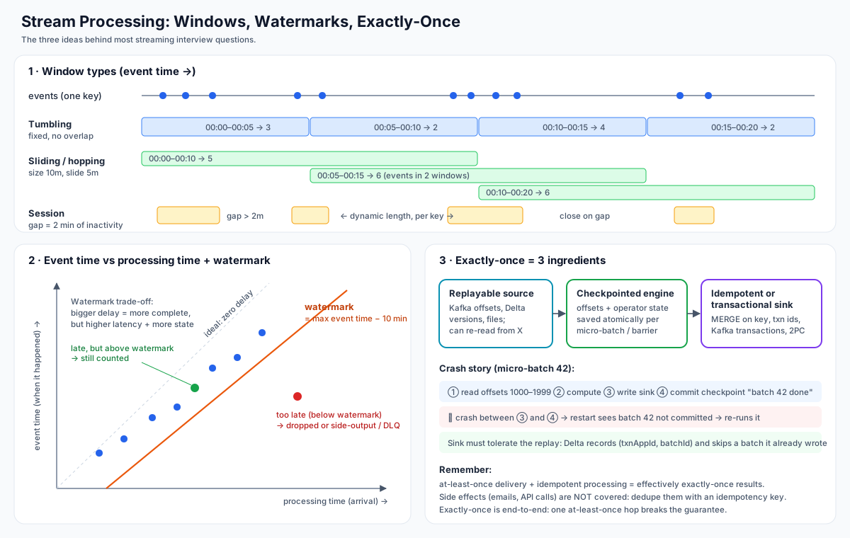
- Event time vs processing time: always aggregate on event time.
- Watermark = “I believe I’ve seen all events up to time T”. Lets the engine finalise windows and drop state.
- Windows: tumbling, sliding/hopping, session.
- Output modes: append (only finalised rows), update (changed rows), complete (whole result).
- Triggers: processing-time interval, available-now (batch-like incremental), continuous.
4. Batch engines
| Engine | Sweet spot |
|---|---|
| Spark | Large-scale ETL, joins over TBs, ML feature pipelines, lakehouse |
| dbt (on a warehouse/Spark) | SQL transformations with tests, docs, lineage, incremental models |
| Warehouse SQL (Snowflake, BigQuery, Databricks SQL, Redshift) | ELT, analytics, BI |
| Trino/Presto | Federated interactive SQL over lakes |
| DuckDB / Polars | Single-node, up to ~100s GB, insanely fast; great for tests and small jobs |
Key batch design rules:
- Idempotent partitions: each run overwrites exactly one logical partition (
INSERT OVERWRITE ... PARTITION (dt='2026-10-01')orMERGE/replaceWhere). - Incremental by default: process only new data (watermark column, Delta CDF, AutoLoader), with a full-refresh escape hatch.
- Deterministic: no
now()inside transformations. Pass the logical date in as a parameter so backfills reproduce history.
5. Storage layer
flowchart TB
    subgraph Catalog["Catalog (Unity / Glue / Polaris / Hive Metastore)"]
        CT[table name → metadata location, permissions]
    end
    subgraph Table["Open table format (Delta / Iceberg / Hudi)"]
        LOG[Transaction log / metadata tree<br/>versions, schema, file list, stats]
    end
    subgraph Files["Object storage (S3 / ADLS / GCS)"]
        F1[part-0001.parquet]
        F2[part-0002.parquet]
        F3[part-0003.parquet]
    end
    CT --> LOG
    LOG --> F1
    LOG --> F2
    LOG --> F3
- Object storage: cheap, infinitely scalable, 11 nines durable, but no transactions, no in-place updates, and listing is slow.
- Parquet: columnar, compressed, with min/max stats per row group → column pruning + predicate pushdown.
- Table format adds: ACID commits, time travel, schema evolution, MERGE/UPDATE/DELETE, file-level stats for data skipping, concurrent writers (optimistic concurrency).
- Deep dive: Storage & table formats.
File-size rule: target 128 MB–1 GB files. Thousands of tiny files are the most common lakehouse performance bug (metadata overhead, task overhead, S3 request costs) → compaction (OPTIMIZE), optimized writes, auto-compaction.
6. Serving stores
The access pattern picks the store:
| Need | Store | Why |
|---|---|---|
| Sub-second slice-and-dice on fresh events, high concurrency (user-facing analytics) | Apache Pinot / Druid / ClickHouse | Columnar + indexes + pre-aggregation (star-tree, rollups), real-time ingestion from Kafka |
| Internal BI, complex SQL, joins, moderate concurrency | Warehouse / lakehouse SQL | Flexible, cheaper per TB, seconds latency |
| Point lookup by key in ms (features, profile, counters) | Redis / DynamoDB / Cassandra / Bigtable | KV, predictable latency, horizontal scale |
| Search, text, logs | Elasticsearch / OpenSearch | Inverted index |
| Similarity search | Vector DB (pgvector, Pinecone, Milvus, Mosaic AI Vector Search) | ANN indexes (HNSW, IVF) |
| Graph traversals | Neo4j / Neptune | Relationships |
| Transactions (source of truth for an app) | Postgres / MySQL | OLTP, ACID |
flowchart LR
    Q{Query pattern?}
    Q -->|"key → value, < 10 ms"| KV[Redis / DynamoDB]
    Q -->|"aggregations on fresh data,<br/>user-facing, 1000s QPS"| OLAP[Pinot / Druid / ClickHouse]
    Q -->|"ad-hoc SQL, joins,<br/>analysts"| WH[Warehouse / Lakehouse SQL]
    Q -->|"nearest neighbours"| VEC[Vector index]
    Q -->|"full text"| ES[Elasticsearch]
Senior nuance: you often need two serving stores: raw history in the lakehouse for flexibility, and pre-aggregated hot data in an OLAP/KV store for latency. Say explicitly which one is the source of truth (usually the lakehouse) and that serving stores can be rebuilt from it.
7. Caches
- Cache-aside (app reads cache, falls back to source, populates cache): default.
- Write-through: write cache + source synchronously (consistency, slower writes).
- TTL for freshness; key design e.g.
metric:{campaign}:{minute}. - In data systems, a cache is mostly used for serving pre-computed aggregates/features, and for dimension lookups inside streaming jobs (broadcast state or async lookups to Redis) to avoid hammering the OLTP DB.
- Pitfalls: thundering herd on expiry (jitter TTLs, request coalescing), cache inconsistency on backfill (invalidate or version keys).
8. Orchestrators
| Airflow | Dagster | Databricks Workflows / Lakeflow Jobs | Prefect | |
|---|---|---|---|---|
| Paradigm | Task DAGs, schedule-centric | Asset-centric (data-aware) | Jobs + tasks, native to the lakehouse | Python flows |
| Strength | Ecosystem, ubiquity | Lineage, partitions, testing | Zero infra, cluster mgmt, DLT/dbt tasks | Dynamic workflows |
| Watch out | Scheduler scale, DAG parsing, XCom misuse | Smaller ecosystem | Vendor-specific | Smaller ecosystem |
Design rules: tasks idempotent, parameterised by logical date, retries with backoff, SLAs/alerts on freshness not just failure, data-aware triggers (run when upstream table updates) over cron chains. More in Orchestration & backfills.
9. Schema registry & contracts
- Central store of Avro/Protobuf/JSON schemas, versioned per subject (topic).
- Compatibility modes:
- BACKWARD (default): new consumers can read old data → you can add fields with defaults or delete fields. Upgrade consumers first.
- FORWARD: old consumers can read new data → add fields, delete optional fields. Upgrade producers first.
- FULL: both.
- Producer serialization fails fast on incompatible change → bad schemas never enter the log.
- Data contract = schema + semantics + SLAs + ownership + quality rules, agreed between producer and consumer and enforced in CI.
10. Probabilistic data structures
| Structure | Answers | Memory | Error | Mergeable? |
|---|---|---|---|---|
| HyperLogLog | Count distinct | ~1.5–12 KB | ~0.8–2% | ✅ (union) → great for rollups |
| Count-Min Sketch | Frequency of item (heavy hitters) | KBs–MBs | Overestimates only | ✅ |
| Bloom filter | ”Have I seen X?” (dedup, join pre-filter) | ~10 bits/item for 1% FP | False positives, no false negatives | ✅ (OR) |
| t-digest / KLL | Percentiles (p50/p95/p99) | KBs | small rank error | ✅ |
| Reservoir sampling | Uniform sample of a stream | k items | exact sample | – |
Use in design: “Real-time unique visitors per page per minute: I’ll store HLL sketches per minute; the hourly/daily numbers are unions of the minute sketches, so I never re-scan raw data. Finance’s exact numbers come from batch.”
SQL examples: approx_count_distinct(user_id), percentile_approx(latency, 0.95), Databricks hll_sketch_agg / hll_union_agg.
Cheat table: “If they say X, reach for Y”
| They say… | Reach for… |
|---|---|
| ”Replay”, “multiple consumers”, “decouple” | Kafka |
| ”Changes from the database” | Log-based CDC (Debezium) → Kafka → MERGE |
| ”Sub-second dashboards for customers” | Pinot/Druid/ClickHouse fed from Kafka |
| ”Exactly once” | Replayable source + checkpoint + idempotent sink; dedup keys |
| ”Late events” | Event-time windows + watermarks + restatement batch |
| ”History of changes” | SCD Type 2 / Delta CDF / snapshots |
| ”Unique users at scale” | HLL sketches |
| ”Top-K trending” | Count-min sketch + heap, or windowed aggregation + rank |
| ”Point lookup features at inference” | Online feature store (Redis/DynamoDB) synced from offline |
| ”Search docs with LLM” | RAG pipeline: chunk → embed → vector index + ACLs |
| ”PII / GDPR” | Classification tags, masking, crypto-shredding, deletion pipeline |